

Re-Examining LayerNorm
Re-Examining LayerNorm
Re-Examining LayerNorm
Conjecture
Dec 1, 2022
This post is part of the work done at Conjecture.
Special thanks to Sid Black, Dan Braun, Carlos Ramón Guevara, Beren Millidge, Chris Scammell, Lee Sharkey, and Lucas Teixeira for feedback on early drafts.
There's a lot of non-linearities floating around in neural networks these days, but one that often gets overlooked is LayerNorm. This is understandable because it's not "supposed" to be doing anything; it was originally introduced to stabilize training. Contemporary attitudes about LayerNorm's computational power range from "it's just normalizing a vector" to "it can do division apparently". And theories of mechanistic interpretability such as features as directions and polytopes are unhelpful, or even harmful, in understanding normalization's impact on a network's representations. After all, normalization doesn't alter the direction of vectors, but it still bends lines and planes (the boundaries of polytopes) out of shape. As it turns out, LayerNorm can be used as a general purpose activation function (you can solve MNIST with a LayerNorm MLP, for example). Concretely, it can do things like this:

and this:

We will explain what's going on in these animations later, but the point is that to develop a strong, principled theory of mechanistic interpretability, we need to grapple with this non-linearity.
In this interactive notebook, we study LayerNorm systematically using math and geometric intuition to characterize the ways in which it can manipulate data. We show that the core non-linearity of LayerNorm can be understood via simple geometric primitives. We explain how these basic primitives may perform semantic operations. For example, folding can be viewed as extracting extremal features (e.g. separating extreme temperatures from normal ones). We leverage these primitives to understand more complex low-dimensional classification tasks with multiple layers of non-linearities. The methods and intuition developed here extend to non-linearities beyond LayerNorm, and we plan to extend them in future work. Below is an interactive summary of the content of the notebook. (If you find the summary interesting, you really should check out the notebook: manipulating the figures helps build geometric intuition.)
Summary
The formula for LayerNorm is something messy like
LayerNorm[x]=x−E[x]√Var[x]+ϵ∗γ+β.
But it turns out the core non-linear operation is (almost) normalizing a vector:
uϵ(x)=x√||x||2+ϵ.
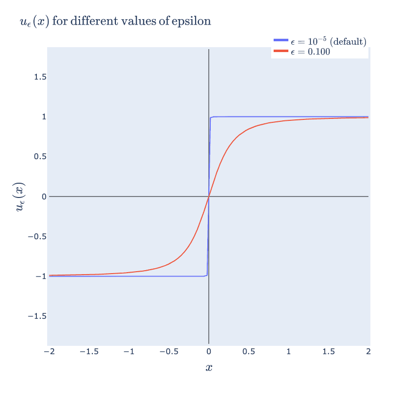
Graphically, this function has the iconic sigmoid shape in one dimension (note that in 1D the norm is simply the absolute value).
Interesting things start happening when we precompose this normalization function with affine transformations (such as scaling and shifting). Below, we start with a collection of points, (x,y), distributed uniformly on the sphere. Then we compute uϵ(tx,y) (stretch/shrink by a factor of t in the x direction and then normalize). Since normalization guarantees points end up on the circle, this operation stretches the distribution along the circle. The right hand panel illustrates how this stretching is captured in the shape of a 1D activation function (the x coordinate of the input against the x coordinate of the output). For example, when t is close to 5, we see that any points with x coordinates not near 0 get compressed towards x=−1 or x=1. This matches the picture in the circle where we see the points bunch up at the left and right sides of the circle.

If we make the same plots with a shifting operation, uϵ(x+t,y), the operation folds the input data.

We can envision possible "semantic" uses for these geometric operations. Stretching can be used to perform an approximate "sign" operation (as in + or - sign). For example, it can take a continuous representation such as a numeric temperature and reduce it to two groups: "hot" vs "cold". Folding can be used to perform an approximate "absolute value" operation. For example, it can be used to separate out extremes from a continuous representation such as temperature and make two groups: "very hot"/"very cold" vs "typical temperature".
The right hand activation plot for folding looks pretty different from typical "activation functions" such as ReLUs or sigmoids. When t is near 2 for example, points with x coordinates near 1 and -1 both get mapped to 1, where points closer to 0 are relaxed away from 1. This gives a characteristic "divet" or, in the language of our semantic explanation, "absolute value" shape. We would not expect this from the 1D activation curve we originally drew. We can explain how this shape arises by instead looking at an activation surface for uϵ in 2D. The various 1D shapes arise as slices of this 2D activation surface. So its the combination

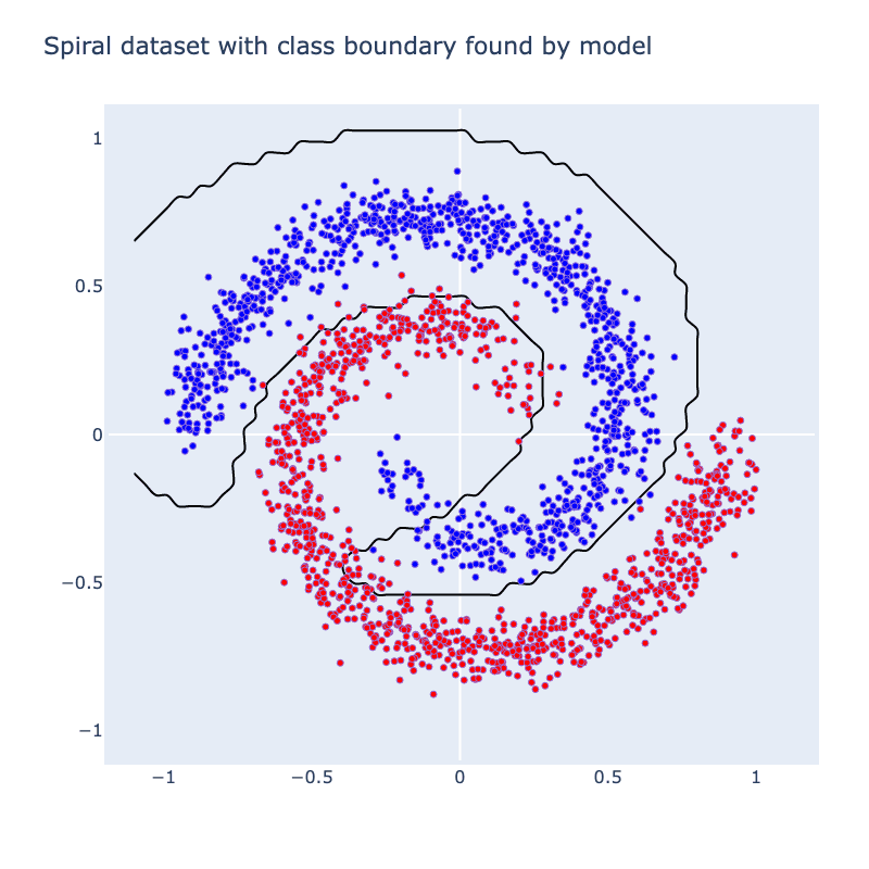
We can now bring our geometric intuition to bear on a small classification task. Below we have 2 classes forming a spiral. We apply a width 3 MLP with uϵ as the activation function (Linear->uϵ->Linear->uϵ->Linear). Below, we've sketched the classification boundary it finds after training.
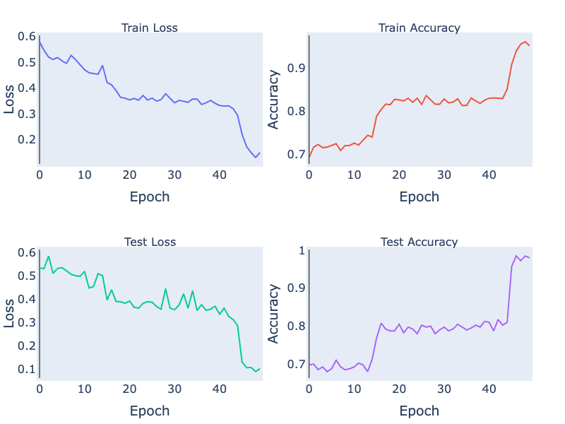
If we check out the loss and accuracy curves, we see evidence of a phase transition. We can speculate on why this occurs. Operations like folding in low dimensions can create sharp changes in the classifier output, since points can move with high-velocity relative to changes in weights (see the 1D folding diagram and note that right before the fold is complete some points are jumping very quickly from one side of the circle to the other). Another possibility is that there are regions in the loss landscape of low, but nonzero, gradients that must be traversed to get to a region of higher gradient where the phase transition happens. It's not clear that the folding and loss gradient explanations are mutually exclusive. In future work, we would like to thoroughly investigate this.
To understand the solution the model found to the task, we can embed the data in 3D and linearly interpolate from layer to layer. Specifically, we interpolate from the raw data to the first activation (output of first uϵ) to the second activation (output of second uϵ). At the end, we rotate the second activation output to aid in visualizing its 3D structure. The neural network has a final separating plane that it applies to construct the class boundary, and we can see roughly where this could go in the visual we have made.

Essentially, the network has turned the dataset into one where there is a blue cap with a red ring around it, which is more-or-less linearly separable. We can have more fun with this set-up. Why not try a harder dataset with more layers? Let's consider this dataset of a sphere divided into 8-parts, where adjacent parts are in opposite classes:

If we run our model the final activation output looks like this:

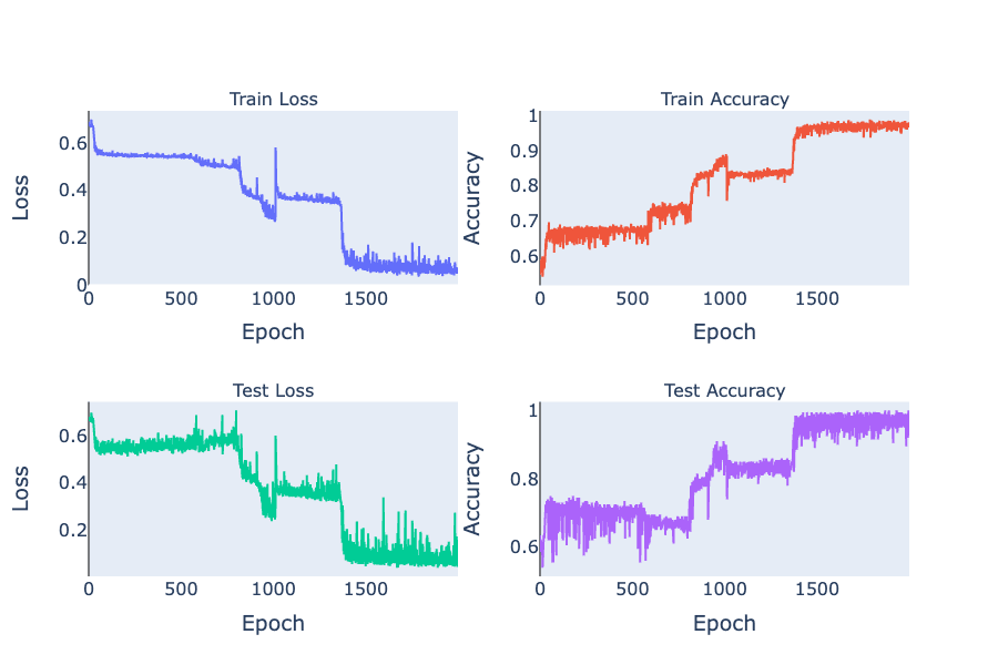
Note that the two classes are now almost linearly separable. To get here, the model has to go through a number of phase transitions and the loss curve looks... weird.
We can reuse our animation method from the spiral example to visualize the way the model is solving this task. We linearly interpolate from the input to the first activation, then the second activation, and so on.

So the model has found an elegant way to fold up the sphere just by using linear and normalization operations! If you've found this interesting, we have a notebook with detailed math and code. In follow-up posts, we plan to look at some variations on this type of analysis and link it to interpreting large models.
From a mechanistic interpretability perspective, we cannot afford to ignore LayerNorm. We may consider finding alternatives to LayerNorm in order to produce models that are better understood by current mechanistic interpretability tools. In the big picture, however, we may have to grapple with the technical difficulties of LayerNorm either way. After all, the core obstacle in understanding LayerNorm is our lack of a theory for mechanistically interpreting non-linear activations. And as long as we cannot account for non-linearities in mechanistic interpretability, we will be unable to robustly explain and constrain the behavior of neural networks. The geometric perspective we have presented here is a step towards a mechanistic theory of non-linear activations that closes the gap in our understanding.
This post is part of the work done at Conjecture.
Special thanks to Sid Black, Dan Braun, Carlos Ramón Guevara, Beren Millidge, Chris Scammell, Lee Sharkey, and Lucas Teixeira for feedback on early drafts.
There's a lot of non-linearities floating around in neural networks these days, but one that often gets overlooked is LayerNorm. This is understandable because it's not "supposed" to be doing anything; it was originally introduced to stabilize training. Contemporary attitudes about LayerNorm's computational power range from "it's just normalizing a vector" to "it can do division apparently". And theories of mechanistic interpretability such as features as directions and polytopes are unhelpful, or even harmful, in understanding normalization's impact on a network's representations. After all, normalization doesn't alter the direction of vectors, but it still bends lines and planes (the boundaries of polytopes) out of shape. As it turns out, LayerNorm can be used as a general purpose activation function (you can solve MNIST with a LayerNorm MLP, for example). Concretely, it can do things like this:

and this:

We will explain what's going on in these animations later, but the point is that to develop a strong, principled theory of mechanistic interpretability, we need to grapple with this non-linearity.
In this interactive notebook, we study LayerNorm systematically using math and geometric intuition to characterize the ways in which it can manipulate data. We show that the core non-linearity of LayerNorm can be understood via simple geometric primitives. We explain how these basic primitives may perform semantic operations. For example, folding can be viewed as extracting extremal features (e.g. separating extreme temperatures from normal ones). We leverage these primitives to understand more complex low-dimensional classification tasks with multiple layers of non-linearities. The methods and intuition developed here extend to non-linearities beyond LayerNorm, and we plan to extend them in future work. Below is an interactive summary of the content of the notebook. (If you find the summary interesting, you really should check out the notebook: manipulating the figures helps build geometric intuition.)
Summary
The formula for LayerNorm is something messy like
LayerNorm[x]=x−E[x]√Var[x]+ϵ∗γ+β.
But it turns out the core non-linear operation is (almost) normalizing a vector:
uϵ(x)=x√||x||2+ϵ.
Graphically, this function has the iconic sigmoid shape in one dimension (note that in 1D the norm is simply the absolute value).

Interesting things start happening when we precompose this normalization function with affine transformations (such as scaling and shifting). Below, we start with a collection of points, (x,y), distributed uniformly on the sphere. Then we compute uϵ(tx,y) (stretch/shrink by a factor of t in the x direction and then normalize). Since normalization guarantees points end up on the circle, this operation stretches the distribution along the circle. The right hand panel illustrates how this stretching is captured in the shape of a 1D activation function (the x coordinate of the input against the x coordinate of the output). For example, when t is close to 5, we see that any points with x coordinates not near 0 get compressed towards x=−1 or x=1. This matches the picture in the circle where we see the points bunch up at the left and right sides of the circle.

If we make the same plots with a shifting operation, uϵ(x+t,y), the operation folds the input data.

We can envision possible "semantic" uses for these geometric operations. Stretching can be used to perform an approximate "sign" operation (as in + or - sign). For example, it can take a continuous representation such as a numeric temperature and reduce it to two groups: "hot" vs "cold". Folding can be used to perform an approximate "absolute value" operation. For example, it can be used to separate out extremes from a continuous representation such as temperature and make two groups: "very hot"/"very cold" vs "typical temperature".
The right hand activation plot for folding looks pretty different from typical "activation functions" such as ReLUs or sigmoids. When t is near 2 for example, points with x coordinates near 1 and -1 both get mapped to 1, where points closer to 0 are relaxed away from 1. This gives a characteristic "divet" or, in the language of our semantic explanation, "absolute value" shape. We would not expect this from the 1D activation curve we originally drew. We can explain how this shape arises by instead looking at an activation surface for uϵ in 2D. The various 1D shapes arise as slices of this 2D activation surface. So its the combination

We can now bring our geometric intuition to bear on a small classification task. Below we have 2 classes forming a spiral. We apply a width 3 MLP with uϵ as the activation function (Linear->uϵ->Linear->uϵ->Linear). Below, we've sketched the classification boundary it finds after training.

If we check out the loss and accuracy curves, we see evidence of a phase transition. We can speculate on why this occurs. Operations like folding in low dimensions can create sharp changes in the classifier output, since points can move with high-velocity relative to changes in weights (see the 1D folding diagram and note that right before the fold is complete some points are jumping very quickly from one side of the circle to the other). Another possibility is that there are regions in the loss landscape of low, but nonzero, gradients that must be traversed to get to a region of higher gradient where the phase transition happens. It's not clear that the folding and loss gradient explanations are mutually exclusive. In future work, we would like to thoroughly investigate this.

To understand the solution the model found to the task, we can embed the data in 3D and linearly interpolate from layer to layer. Specifically, we interpolate from the raw data to the first activation (output of first uϵ) to the second activation (output of second uϵ). At the end, we rotate the second activation output to aid in visualizing its 3D structure. The neural network has a final separating plane that it applies to construct the class boundary, and we can see roughly where this could go in the visual we have made.

Essentially, the network has turned the dataset into one where there is a blue cap with a red ring around it, which is more-or-less linearly separable. We can have more fun with this set-up. Why not try a harder dataset with more layers? Let's consider this dataset of a sphere divided into 8-parts, where adjacent parts are in opposite classes:

If we run our model the final activation output looks like this:

Note that the two classes are now almost linearly separable. To get here, the model has to go through a number of phase transitions and the loss curve looks... weird.

We can reuse our animation method from the spiral example to visualize the way the model is solving this task. We linearly interpolate from the input to the first activation, then the second activation, and so on.

So the model has found an elegant way to fold up the sphere just by using linear and normalization operations! If you've found this interesting, we have a notebook with detailed math and code. In follow-up posts, we plan to look at some variations on this type of analysis and link it to interpreting large models.
From a mechanistic interpretability perspective, we cannot afford to ignore LayerNorm. We may consider finding alternatives to LayerNorm in order to produce models that are better understood by current mechanistic interpretability tools. In the big picture, however, we may have to grapple with the technical difficulties of LayerNorm either way. After all, the core obstacle in understanding LayerNorm is our lack of a theory for mechanistically interpreting non-linear activations. And as long as we cannot account for non-linearities in mechanistic interpretability, we will be unable to robustly explain and constrain the behavior of neural networks. The geometric perspective we have presented here is a step towards a mechanistic theory of non-linear activations that closes the gap in our understanding.
This post is part of the work done at Conjecture.
Special thanks to Sid Black, Dan Braun, Carlos Ramón Guevara, Beren Millidge, Chris Scammell, Lee Sharkey, and Lucas Teixeira for feedback on early drafts.
There's a lot of non-linearities floating around in neural networks these days, but one that often gets overlooked is LayerNorm. This is understandable because it's not "supposed" to be doing anything; it was originally introduced to stabilize training. Contemporary attitudes about LayerNorm's computational power range from "it's just normalizing a vector" to "it can do division apparently". And theories of mechanistic interpretability such as features as directions and polytopes are unhelpful, or even harmful, in understanding normalization's impact on a network's representations. After all, normalization doesn't alter the direction of vectors, but it still bends lines and planes (the boundaries of polytopes) out of shape. As it turns out, LayerNorm can be used as a general purpose activation function (you can solve MNIST with a LayerNorm MLP, for example). Concretely, it can do things like this:

and this:

We will explain what's going on in these animations later, but the point is that to develop a strong, principled theory of mechanistic interpretability, we need to grapple with this non-linearity.
In this interactive notebook, we study LayerNorm systematically using math and geometric intuition to characterize the ways in which it can manipulate data. We show that the core non-linearity of LayerNorm can be understood via simple geometric primitives. We explain how these basic primitives may perform semantic operations. For example, folding can be viewed as extracting extremal features (e.g. separating extreme temperatures from normal ones). We leverage these primitives to understand more complex low-dimensional classification tasks with multiple layers of non-linearities. The methods and intuition developed here extend to non-linearities beyond LayerNorm, and we plan to extend them in future work. Below is an interactive summary of the content of the notebook. (If you find the summary interesting, you really should check out the notebook: manipulating the figures helps build geometric intuition.)
Summary
The formula for LayerNorm is something messy like
LayerNorm[x]=x−E[x]√Var[x]+ϵ∗γ+β.
But it turns out the core non-linear operation is (almost) normalizing a vector:
uϵ(x)=x√||x||2+ϵ.
Graphically, this function has the iconic sigmoid shape in one dimension (note that in 1D the norm is simply the absolute value).

Interesting things start happening when we precompose this normalization function with affine transformations (such as scaling and shifting). Below, we start with a collection of points, (x,y), distributed uniformly on the sphere. Then we compute uϵ(tx,y) (stretch/shrink by a factor of t in the x direction and then normalize). Since normalization guarantees points end up on the circle, this operation stretches the distribution along the circle. The right hand panel illustrates how this stretching is captured in the shape of a 1D activation function (the x coordinate of the input against the x coordinate of the output). For example, when t is close to 5, we see that any points with x coordinates not near 0 get compressed towards x=−1 or x=1. This matches the picture in the circle where we see the points bunch up at the left and right sides of the circle.

If we make the same plots with a shifting operation, uϵ(x+t,y), the operation folds the input data.

We can envision possible "semantic" uses for these geometric operations. Stretching can be used to perform an approximate "sign" operation (as in + or - sign). For example, it can take a continuous representation such as a numeric temperature and reduce it to two groups: "hot" vs "cold". Folding can be used to perform an approximate "absolute value" operation. For example, it can be used to separate out extremes from a continuous representation such as temperature and make two groups: "very hot"/"very cold" vs "typical temperature".
The right hand activation plot for folding looks pretty different from typical "activation functions" such as ReLUs or sigmoids. When t is near 2 for example, points with x coordinates near 1 and -1 both get mapped to 1, where points closer to 0 are relaxed away from 1. This gives a characteristic "divet" or, in the language of our semantic explanation, "absolute value" shape. We would not expect this from the 1D activation curve we originally drew. We can explain how this shape arises by instead looking at an activation surface for uϵ in 2D. The various 1D shapes arise as slices of this 2D activation surface. So its the combination

We can now bring our geometric intuition to bear on a small classification task. Below we have 2 classes forming a spiral. We apply a width 3 MLP with uϵ as the activation function (Linear->uϵ->Linear->uϵ->Linear). Below, we've sketched the classification boundary it finds after training.

If we check out the loss and accuracy curves, we see evidence of a phase transition. We can speculate on why this occurs. Operations like folding in low dimensions can create sharp changes in the classifier output, since points can move with high-velocity relative to changes in weights (see the 1D folding diagram and note that right before the fold is complete some points are jumping very quickly from one side of the circle to the other). Another possibility is that there are regions in the loss landscape of low, but nonzero, gradients that must be traversed to get to a region of higher gradient where the phase transition happens. It's not clear that the folding and loss gradient explanations are mutually exclusive. In future work, we would like to thoroughly investigate this.

To understand the solution the model found to the task, we can embed the data in 3D and linearly interpolate from layer to layer. Specifically, we interpolate from the raw data to the first activation (output of first uϵ) to the second activation (output of second uϵ). At the end, we rotate the second activation output to aid in visualizing its 3D structure. The neural network has a final separating plane that it applies to construct the class boundary, and we can see roughly where this could go in the visual we have made.

Essentially, the network has turned the dataset into one where there is a blue cap with a red ring around it, which is more-or-less linearly separable. We can have more fun with this set-up. Why not try a harder dataset with more layers? Let's consider this dataset of a sphere divided into 8-parts, where adjacent parts are in opposite classes:

If we run our model the final activation output looks like this:

Note that the two classes are now almost linearly separable. To get here, the model has to go through a number of phase transitions and the loss curve looks... weird.

We can reuse our animation method from the spiral example to visualize the way the model is solving this task. We linearly interpolate from the input to the first activation, then the second activation, and so on.

So the model has found an elegant way to fold up the sphere just by using linear and normalization operations! If you've found this interesting, we have a notebook with detailed math and code. In follow-up posts, we plan to look at some variations on this type of analysis and link it to interpreting large models.
From a mechanistic interpretability perspective, we cannot afford to ignore LayerNorm. We may consider finding alternatives to LayerNorm in order to produce models that are better understood by current mechanistic interpretability tools. In the big picture, however, we may have to grapple with the technical difficulties of LayerNorm either way. After all, the core obstacle in understanding LayerNorm is our lack of a theory for mechanistically interpreting non-linear activations. And as long as we cannot account for non-linearities in mechanistic interpretability, we will be unable to robustly explain and constrain the behavior of neural networks. The geometric perspective we have presented here is a step towards a mechanistic theory of non-linear activations that closes the gap in our understanding.
Latest Articles



Dec 2, 2024
Conjecture: A Roadmap for Cognitive Software and A Humanist Future of AI
Conjecture: A Roadmap for Cognitive Software and A Humanist Future of AI
An overview of Conjecture's approach to "Cognitive Software," and our build path towards a good future.


Feb 24, 2024
Christiano (ARC) and GA (Conjecture) Discuss Alignment Cruxes
Christiano (ARC) and GA (Conjecture) Discuss Alignment Cruxes
The following are the summary and transcript of a discussion between Paul Christiano (ARC) and Gabriel Alfour, hereafter GA (Conjecture), which took place on December 11, 2022 on Slack. It was held as part of a series of discussions between Conjecture and people from other organizations in the AGI and alignment field. See our retrospective on the Discussions for more information about the project and the format.


Feb 15, 2024
Conjecture: 2 Years
Conjecture: 2 Years
It has been 2 years since a group of hackers and idealists from across the globe gathered into a tiny, oxygen-deprived coworking space in downtown London with one goal in mind: Make the future go well, for everybody. And so, Conjecture was born.
Sign up to receive our newsletter and
updates on products and services.
Sign up to receive our newsletter and updates on products and services.
Sign up to receive our newsletter and updates on products and services.